Shackleton – Imperial Trans-Antarctic Expedition Map

Recently I’ve been reading Endurance: Shackleton’s Incredible Voyage. On the whole book they describe its current position, movement, etc.. but it’s difficult for me to understand certain positions on the poles. Also, the history is so astonishing that it deserved a cool map.

There are some maps of the Imperial Trans-Antartcic Expedition: http://www.kodak.com, http://www.wgbh.org, coolAntarctica, and a long etcetera. But I wanted to play a little bit.

Results

Online Map:
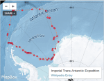
Nice view of Shackleton Imperial Trans-Antartcic expedition. Information of each point and also photos.

Interactive Shackleton Map at MapBox

Images:

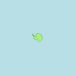
Shackleton Map

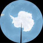
Shackleton Map (closer)

Process

>>Software

To create this maps I used:

• Qgis
• GDAL
• TileMill

>>Data

A combination of data sets is employed. First of all, I obtained the Shackleton data set from Shackleton’s expedition, Endurance, Antarctica google group. The raster background and the graticule comes from NaturalEarthData. The Antarctica outline is provided by the Antarctic Digital Database (you have to register to access the data). South Georgia outline from Global Administrative Areas. Finally, the ice sea extent comes from National Snow and Ice data center.

The ice dataset represents 1979 while the expedition took place on 1914. It felt important to show the ice sea coverage, thus I decided to add this temporary inaccurate data that fits quite well with the description of the expedition.

>>Processing

For this project, I work with EPSG:3031 projection (WGS 84 / Antarctic Polar Stereographic), consequently I’ll save all the shapefiles using this projection.

Raster: The raster provided is projected as EPSG:4326. The objective is to use gdal_warp to obtain a properly projected geoTiff.
A little bit of trouble appear on this point, reprojecting the 167M file results in a 1,5G file that is unmanageable. To avoid that, first I crop the original file to match only the Antarctica:

gdal_merge.py -ul_lr -180.0 -50.0 180.0 -90.0 -of GTiff -o NE1_50M_SR_W_cropAntarctica.tif NE1_50M_SR_W.tif


World Raster EPSG:4236

Antarctica Raster EPSG:4236

next step, reproject:

gdalwarp -ts 10000 10000 -wo "SAMPLE_STEPS=1000 SAMPLE_GRID=YES" -s_srs EPSG:4326 -t_srs EPSG:3031 -of GTiff NE1_50M_SR_W_cropAntarctica.tif Antarctica_epsg3031.tiff


With -ts the filesize is specified to avoid a big file result, and with -wo some specific gdalwarp options are defined:

SAMPLE_GRID=YES/NO: Setting this option to YES will force the sampling to include internal points as well as edge points which can be important if the transformation is esoteric inside out, or if large sections of the destination image are not transformable into the source coordinate system.

SAMPLE_STEPS: Modifies the density of the sampling grid. The default number of steps is 21. Increasing this can increase the computational cost, but improves the accuracy with which the source region is computed.
— gdal warp manual

This options are important to obtain a clean image:

Default Warp

Warp with SAMPLE_STEPS = 200

Warp with SAMPLE_STEPS = 1000

Shackleton Route: This is provided as a KMZ. I unpack the KMZ and open the resulting KML with Qgis. From Qgis I save the route as a shapefile with the EPSG:3031 projection. Note that TileMill can load KML, but KML only supports EPSG:4326, that’s the reason why I store the data in other formats.

Shackleton Points: This made me lose some time. The points contain a title and HTML information. If you save as shapefile, there’s a limit of 80 character imposed (you can increase it, but not enough) because of the dbf file format. I tried to save SpatiaLite and GML, but then TileMill refused to open it (for some reason.. Qgis, TileMill.. I don’t know). The final solution is to save a geoJSON that tileMill can open with no problem, and there’s no data missing.

Ice Coverage:
The ice coverage is a shapefile with various polygons. I deleted all the polygons representing Antarctica obtaining a big polygon with the ice sea. This polygon covers also Antarctica, but I don’t want it in my result, I want a polygon with a Hole where Antarctica is. Polygon difference is the only step needed, and this can be directly performed from Qgis with ftools plugin.

Graticule:
To obtain the graticule no process is needed, I simply save it with the correct projection.

Labeling: The labels are defined manually. I create Various Line shapefiles with two attributes (id:int, label:string). The idea is that tilemill will render the names following the lines defined.

Qgis Shapefiles for Labelling

>>TileMill

TileMill automatically reprojects the layers, but I don’t want the big Antarctica represented by ‘web mercator’ projection. The trick here is to configure all the layers in tilemill as EPSG 3857 (a specific web mapping projection).

Proj4 code of the EPSG 3857 projection:

+proj=merc +lon_0=0 +k=1 +x_0=0 +y_0=0 +a=6378137 +b=6378137 +towgs84=0,0,0,0,0,0,0 +units=m +no_defs


Tilemill Antarctica Reprojected

Tilemill Antarctica when defined as 3857

Basic TileMill Styling code

Map {
  background-color: #000;
}

#sgeorgia {
  line-color:#89cbd5;
  line-width:1;
  polygon-opacity:0.9;
  polygon-fill:#DDD;
}

#Antarctica {
  polygon-opacity:0.2;
  polygon-fill:#89cbd5;
  [cst01srf="land"] {polygon-fill:#fff;}
  [cst01srf="ocean"] {polygon-fill:#89cbd5;}
  [cst01srf="ice shelf"] {polygon-fill:#89cbd5;}
  [cst01srf="ice tongue"] {polygon-fill:#89cbd5;}
}

#shackletonroute {
  line-width:2;
  line-color:#f3865a;
  line-dasharray: 4,4;
}

#shackletonpoints [zoom>3]{
  marker-width:3;
  marker-fill:#f45;
  marker-line-color:#813;
  marker-allow-overlap:true;
}


#ne150msrwantartic100 {
  raster-opacity:1;
}

#graticule {
  line-width:0.5;
  line-color:#555;
  line-dasharray: 2,2;
}

#icesea1979clipped {
  line-color:#fff;
  line-width:0.5;
  polygon-opacity:0.2;
  polygon-fill:#fff;
}

Labeling code:

@font_reg: "Ubuntu Regular","Arial Regular","DejaVu Sans Book";
@title_reg: "Ubuntu Regular";

.genericlabel{
  text-name:"[name]";
  text-face-name:@font_reg;
  text-fill:#036;
  text-size:20;
  text-halo-radius:1;
  text-halo-fill:rgba(255,255,255,0.75);
  text-wrap-width:30;
  text-line-spacing:2;
  text-placement:line;
 }

.genericlabel #oceanlabels{
  text-size:20;
  [zoom > 5]{
    text-size:40;
  }
}

.genericlabel #weddellsealabel{
  text-name:"[label]";
  text-size:15;
  [zoom > 5]{
    text-size:30;
  }
}

.shackletonpoints [zoom>4] {
  text-name:"[Name]";
  text-face-name:@font_reg;
  text-fill:#036;
  text-dx: 7;
  text-placement-type: simple;
  text-size:10;
  text-halo-radius:1;
  text-halo-fill:rgba(255,255,255,0.75);
  text-wrap-width:30;
  text-line-spacing:2;
  }

.Antarcticalabelline {
  text-name:"[label]";
  text-face-name:@title_reg;
  text-fill:#000;
  text-placement:line;
  text-size:30;
  text-character-spacing: 50;
  text-halo-radius:1;
  text-halo-fill:rgba(125,125,125,0.75);
  [zoom > 5]{
    text-size:50;
  }
  }

.graticule{
  text-name:"[display]";
  text-face-name:@font_reg;
  text-placement: line;
}

Closing comments

It seemed easy and fast, but I spent some time on this map. Still there are some things that I don’t like, and maybe try to fix on the future.

MapBox Tiling Errors

<style>
.wax-tooltip {
  max-width: 400px !important;
}
</style>
{{{Description}}}